An Introduction to Geo Indexes and their performance characteristics: Part I

Starting with the mass-market availability of smartphones and continuing with IoT devices, self-driving cars ever more data is generated with geo information attached to it. Analyzing this data in real-time requires the use of clever indexing data-structures. Geo data in ArangoDB consists of 2 or more dimensions representing (x, y) coordinates on the earth surface. Searching on a single number is essentially a solved problem, but effectively searching on multi-dimensional data can be more difficult as standard indexing techniques cannot be used.

There exist a variety of indexing techniques. In this blogpost Part I, I will introduce some of the necessary background knowledge required to understand the ArangoDB geo index data structure. First I will start by introducing quadtrees and then I will extend this concept to geohashes and space filling curves like the Hilbert curve. Next week, I will publish Part II including details about the ArangoDB geo index implementation and performance benchmarking.

Basics

In this first section I will introduce some of the basics used in the ArangoDB geo index, starting from quadtrees. This should give you some of the necessary background information to understand the following section. This section was partially adapted from two great blogpost from Nick Johnson and Peter Karich.

QuadTree

In computer science a Tree is a fundamental data structures used in all kinds of different applications. It allows us to group data into hierarchies in which a search algorithm can easily find values in O(log(n)) time.

A quadtree is of course just a tree where each internal node has four children. Quadtrees are often used to recursively sub-divide two-dimensional spaces into smaller regions. This is exactly the way quadtrees can be used for indexing geospatial information: A leaf node will contain several indexed points (coordinates), an internal node will have four children one for each quadrant spanned by the axes.

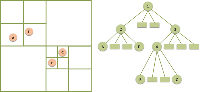
On inserting a datapoint a search algorithm will walk down the quadtree from the root and decide at each internal point in which quadrant a point should belong. Once the algorithm arrives at a leaf, the point can be inserted in the list of points (or split the leaf if the number of points exceeds some defined maximum).

A query for a geo index usually consists of some area for which we would like to retrieve
all points which are contained in it. This can simply be accomplished by starting at the root
and recursively checking for each child node, if the query area intersects with the quadrant contained by the child node. Once one arrives at a leaf, just check if the points intersect with the query area and return them if they do.

Space filling curves

One property of the quadtree is that for any given set of points and tree depth, the resulting quadtree will always look very similar. If you set the depth (height) of the quadtree in the beginning, you will be able to know the resulting leaf node for every point / coordinate without ever constructing the actual tree. This essentially allows us to compute a number for each coordinate with a fixed width, essentially similar to the geohash method (I will call them geostrings to avoid confusion). These geostrings can essentially be computed by interleaving the bits of the latitude and longitude (x, y) values. You can see a nice visualization of this in the next image:

Now we can disregard the actual quadtree entirely and just work with a list of single values for each point. Lookups in a sorted list are possible in O(log(n)), but we also need to be able to efficiently find entire areas (ranges) in this list.

A very inefficient query implementation can perform a scan on the range of possible geostrings and check each point contained in the range. This would not be an efficient query, because we would scan large areas which can actually be completely discarded. The essence of fast querying in databases is rejecting as many wrong possible results very fast. Without the quadtree we cannot easily decide anymore which ranges of the list we need to scan. Luckily the equivalent of the internal quadtree nodes are now the common prefixes of the geohashes. Each geostring-prefix will essentially define a range of geostrings to scan.

Now we need to construct a set of prefixes which fulfill these requirements:

1. The prefix set completely covers the query region.
2. Includes as little coordinates outside the query region as possible
3. Minimize the number of ranges which are not adjacent (Seeks are expensive)

A query can scan over all geostrings starting with one of the prefixes in the prefix set and compute the result. The above image shows the set of (green) quadrants identified by an optimal set of prefixes for the query (search area is the circle). The way in which we interleaved the coordinates to get our geostring now dictates the order in which quadrants are visited by a scan.

In the sketches above we numbered our quadrants in a left-right / top-bottom order. This means we will have to visit the quadrants following a “Z-Curve” (shown on the image). As you can easily see there is a discontinuity there, which prevents us from merging most ranges in which we want to look for coordinates. Only the two ranges in the bottom right of the selected area can actually be merged, yet all of these quadrants are adjacent.

One idea to increase the number of adjacent scanning ranges is to just rearrange the order in which the quadrants will be visited. The order should for example resemble a “U” shape and should always allow us to match a quadrant up with neighboring quadrants. This way expensive “seek” operations in the list of geostrings can be avoided. The order in which quadrants would be visited is shown in the next sketch:

It is not super important for the next parts of the article to understand how exactly the Hilbert curve is drawn. For all intents and purposes all the Hilbert curve provides for us is a way to order points on a 2D-plane more efficiently. Previously we just interleaved the bits of the coordinates similar to (lat 1, long 1, lat 2, long 2). Now we can use the Hilbert curve recursively to determine the quadrant to visit next.

ArangoDBs Geo Queries

ArangoDB currently supports two main ways to use the geo index in AQL queries, you can easily try these out by downloading the binary from https://www.arangodb.com/download-major for your prefered OS (free & open source).

Let’s consider the following use-case. You want to find all restaurants in a given radius around a given position. Maybe for a map overlay or a location aware mobile app.

1. Find points within circle or square area around a target point (AQL function `WITHIN`)

Pre ArangoDB 3.2 such a query would have to look like this:

  FOR doc IN WITHIN(coll, targetLat, targetLon, 1000, "dist")
    RETURN doc

Below you can see the result of such a query as a map overlay. The red pointers visualize a found restaurant within a given radius around a given point in space.

One can already do a few interesting things with these functions but of course there is more fancy stuff people want to do with geo-locations.

Starting from 3.2 the equivalent query can use a `FILTER` statement and the optimizer will take care of making it use the geo index:

  FOR doc IN coll
    FILTER DISTANCE(doc.lat, doc.lon, targetLat, targetLon) < 1000
    RETURN doc

2. Query points around a target coordinate in increasing order of distance (AQL function `NEAR` or through the geocursor)

Pre ArangoDB 3.2 an example query for points near `target` coordinates using the `NEAR` AQL function could look like this:

  FOR doc IN NEAR(coll, targetLat, targetLon, 100)
    RETURN doc

Explicitly using the `NEAR` function is the legacy pre 3.2 method to write such a query. Starting from ArangoDB 3.2 essentially the same query can be written by combining the `SORT` keyword with the `DISTANCE` function. The combination will automatically be detected and converted to use the geo index via the so called geo-cursor:

  FOR doc IN coll
    SORT DISTANCE(targetLat, targetLon, doc.lat, doc.lon) ASC
    LIMIT 100
    RETURN doc

Another add-on to the geo functionalities in ArangoDB 3.2 is that one can now apply additional FILTER conditions on arbitrary attributes to geo queries. For example one not only wants to find all restaurants in a given radius but rather all vegetarian restaurants or restaurants with more than 4 out of 5 stars in a ranking.

The result of a query using a FILTER condition in a map overlay could look like the image below. The green pointers show the restaurant meeting the FILTER condition while the red ones would be filtered out.

You can try the new geo_cursor in ArangoDB yourself by following this tutorial or you can get a simple demonstration here.

One can verify the use of the index within an AQL statement by using the `db._explain` command:

// explain query
arangod> db._explain(q)
Query string:
 FOR doc IN coll SORT distance(targetLat,targetLon,doc.lat,doc.lon) 
                      ASC LIMIT 1000 RETURN d
 
Execution plan:
 Id   NodeType        Est.   Comment
  1   SingletonNode      1   * ROOT
  7   IndexNode       4443     - FOR doc IN coll   /* geo2 index scan */
  5   LimitNode          1       - LIMIT 0, 1000
  6   ReturnNode         1       - RETURN doc
 
Indexes used:
 By   Type   Collection      Unique   Sparse   Selectivity   Fields             Ranges
  7   geo2   places_to_eat   false    true             n/a   [ "lat", "lon" ]   NEAR(doc, targetLat, targetLon)
 
Optimization rules applied:
 Id   RuleName
  1   geo-index-optimizer
  2   remove-unnecessary-calculations-2

In this Part I, I tried to provide the theoretical background of different geo index techniques and show the current possibilities with ArangoDBs geo index and geo-cursor.

Continue with Part II, which focuses mostly on the actual geo index implementation in ArangoDB and a performance comparison of ArangoDB and VP-Tree based indexes.