Entity Resolution in ArangoDB

Estimated reading time: 8 minutes

This post will dive into the world of Entity Resolution in ArangoDB.  This is a companion piece for our Lunch and Learn session, Graph & Beyond Lunch Break #15: Entity Resolution.

In this article we will:

• give a brief background in Entity Resolution (ER)
• discuss some use-cases for ER
• discuss some techniques for performing ER in ArangoDB

What is Entity Resolution?

Entity Resolution is the process of disambiguating records of real-world entities that are represented multiple times in a database or across multiple databases.  

An entity is a unique thing (person, company, product etc.) in the real world with a set of attributes that describes it (a name, zip/postal code, gender, deviceID,  title, price, product category, etc) . The single entity might have multiple references across multiple data sources.  For example, a single user might have two different email addresses, a company might have multiple phone numbers in CRM and ERP systems. Many real-world datasets do not contain unique identifiers.  In such cases, we have to use a combination of fields to identify unique entities across records by grouping or linking them together.

Entity Resolution (ER) is a process akin to data deduplication that aims to uniquely resolve data that potentially comes from multiple sources, to a single real-world entity.  The applications for entity resolution are wide and varied across industry verticals including fraud detection, KYC, recommendations engine, and customer 360, just to name a few.  

Entity Resolution is an ideal use-case for a graph database like ArangoDB. In subsequent sections, we will discuss the steps to take and things to consider when you build ER applications with ArangoDB.

Entity Resolution in ArangoDB – first, build a graph

The first step is to create a graph to represent the entities you wish to resolve and their corresponding attributes.  Data can be read in from a CSV file, perhaps ETL’ed from multiple data sources.  Here’s how a sample schema would look like for ER.

_{figure 1}

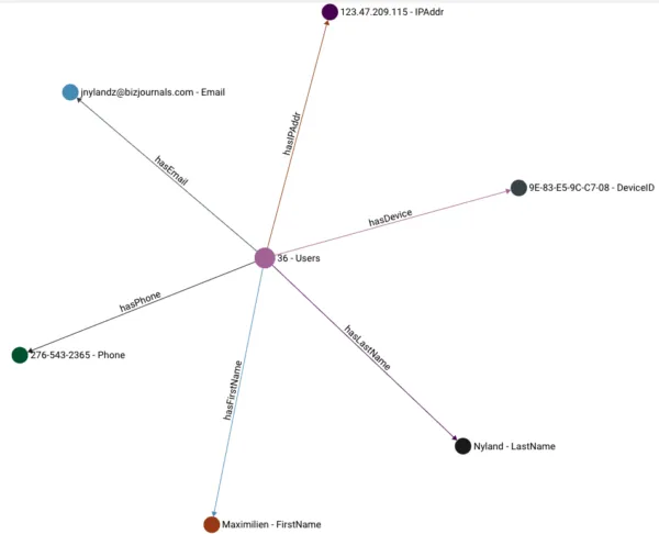
In this example, the entity is a user with attributes like first name, last name, ip address, email, phone and device ID.  These are represented as vertices and edges connecting the entity to its attributes.  As the graph gets populated, we will start to see attributes that are shared by multiple entities.

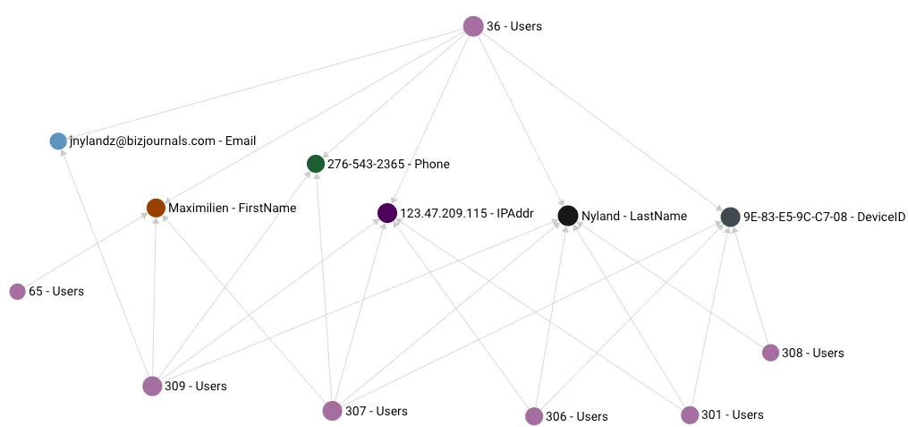
_{^{Figure 2}}

The subgraph above shows multiple user entities with a number of shared attributes, as shown by the edges.  You can see User 309 and User 36 share a total of 5 attributes in common (email, first name, phone, ip address and last name) whereas User 308 only shares 2 attributes with User 36.

Modeling the data like this in a graph makes it very easy to look for matching attributes between users.  As we will see in the next section, matching attributes between users is key when you are looking for similarities between them.

Computing similarity between entities

At the heart of any entity resolution task or algorithm is the computation of similarity.  

How similar is User 36 compared to User 309?  Which users amongst User 65, 309, 307, 306, 301, and 308 are most similar to User 36?  The ability to answer these questions will allow you to build a probabilistic graph that can be used for more graph analytics downstream.

One can utilize the typical similarity algorithms like Jaccard or Cosine similarity in ArangoDB. Or perhaps you need something custom that is domain specific.  All these can be achieved and expressed in AQL (ArangoDB Query Language).

Example 1 – Find Similar Users using Jaccard in AQL

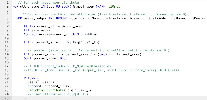
^{_{Please refer to Figure 1 above for the graph schema.}}

Before we dive into the AQL, please note that you can calculate Jaccard index, using the built-in AQL function for the Array data type.

However, we are calculating Jaccard manually here on line 14, since the nature of our 2-hop traversal gives us the intersection set and it’s inexpensive to get the cardinality (line 11). Furthermore, the cardinality of both setA (input_user’s set of attributes) and setB is fixed at 6 (hasLastName, hasFirstName, hasEmail, hasIPAddr, hasPhone, hasDevice), assuming the data is clean.

Executing the above AQL function with a value of “Users/36” for @input_user gives the following result.

The result is a list of users most similar to ‘Users/36’ in descending order of their computed jaccard values.

Uncommenting lines 17, we can supply a threshold like “0.7” to filter out users with a jaccard value less than 0.7.  Re-running with a @threshold value of “0.7” will return only the top 2 rows from previous result (i.e. Users/307 and Users/309).

Grouping or Linking Together Similar Users

Now that we matched and calculated which entities are most similar amongst themselves, the last step in building out our probabilistic graph is to group or link similar entities together. One approach is to create an edge between 2 similar entities and store the computed jaccard value as an attribute on the edge.

In our example above, this is achieved by uncommenting line 18.

INSERT {_from: userBs, _to: @input_user, similarity: jaccard_index} INTO sameAs

This will create new sameAs edges between users most similar (userBs) to our input_user.

Re-running the AQL function will result in the following graph with ‘sameAs’ edges added for Users/307 and Users/309.

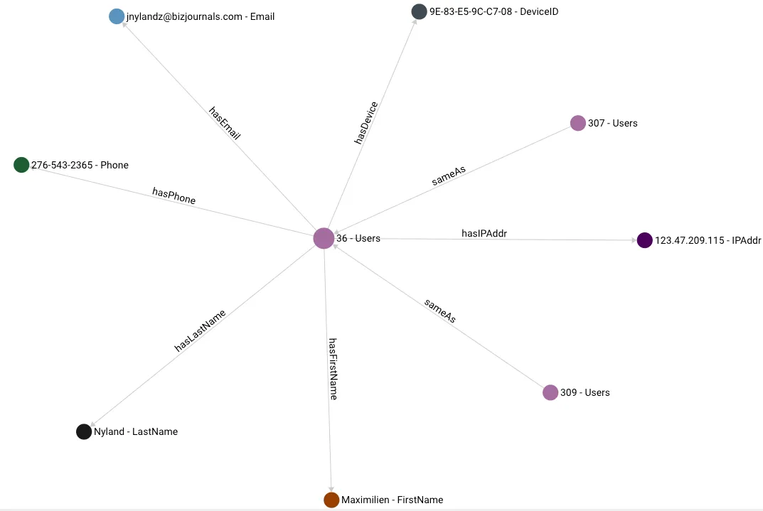
In this example we are using an INSERT to populate the sameAs edge.  In real life, you probably want to do an UPSERT instead.  An UPSERT will insert if the edge is not there, otherwise it will perform an update.

Finding the Right Similarity Algorithm

While Jaccard Similarity might be good enough for certain domains and use-cases it does not differentiate between the types of attributes.  Let’s see how Jaccard is computed.

It treats all attributes with equal weight. You can compute Jaccard by knowing the cardinalities of 3 sets.  Jaccard does not differentiate between a last name match versus a match on device IDs.  In our example, we can argue that a match on device ID is actually worth more than a match on last names.

In some cultures, you find very common last names.  For example, the last name “Singh” in India, there are alot of people with that last name.  Or first name “David”.  On the other hand, a device ID uniquely identifies a specific mobile device.  So we can say a match on device ID should be given a heavier weighting compared to a match on last name.

In the next AQL example, we show a custom similarity algorithm that assigns different weights for different attribute types.

Example 2 – Find Similar Users using a custom algorithm

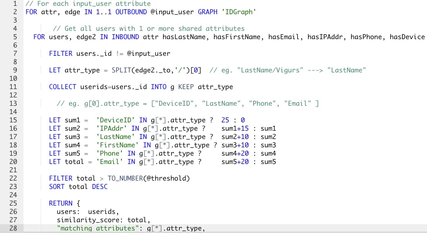
^{Please refer to Figure 1 above for the graph schema.}

In this example, we are doing the same 2-hop traversal pattern as in example 1.  What’s different is we are aggregating on the types of attributes.  We then process the aggregated attribute types to assign different weights for each attribute type.  We assign a weight of 25 for a deviceID match, a weight of 15 for IP Address match, 10 for last name, etc.  Finally, we compute the total sum of the weights for all matched attribute types.  This sum is then used as the similarity value.
Running the above query with @input_user “Users/36” and a @threshold value of 50 will give the following result.

Now Users/307 has a higher similarity score than Users/309 because it has a match on DeviceID.  Using Jaccard in example 1, both these users have similar jaccard values.

Next Steps

In this tutorial we’ve learned how to do Entity Resolution in ArangoDB.  We showed examples on how to build a probabilistic graph for your entities.  If you would like to continue learning more about ArangoDB, here are some next steps to get you started!

• Get a 2 week free Trial with the ArangoDB Cloud
• Download ArangoDB
• ArangoDB Training Center
• Getting Started with ArangoDB – Udemy

Continue Reading

ArangoML Series: Multi-Model Collaboration

State of the Art Preprocessing and Filtering with ArangoSearch

ArangoML Series: Intro to NetworkX Adapter